Differential equations

Odesolve: write the equation as it is

A mass on a spring, with a little damping:

As text

M := 2 kg
k := 50 N/m
c := 1 N*s/m
given
x''(t) == -(k*x(t) + c*x'(t))/M
x(0 s) == 0.1 m
x'(0 s) == 0 m/s
x := Odesolve(t, 5 s)
x(1 s) = ?
x(5 s) = ?

Open this example · Download .bbm

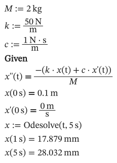
• Below given, write the equation using the variable (t), and the starting values at a number (x(0 s) == 0.1 m). Derivatives are written with primes, x'(t) and x''(t).
• Odesolve(t, 5 s) solves from the starting point to 5 s, and gives the unknown as a function: x(1 s), or plot it.
• Units are checked: here the starting values give x its unit and t its unit, and each side of the equation must agree.
• The highest derivative needn’t be on its own: Beermat finds it from the equation.

Careful with names: the mass above is M, because m := 2 kg would make m a mass instead of the metre for everything below it.

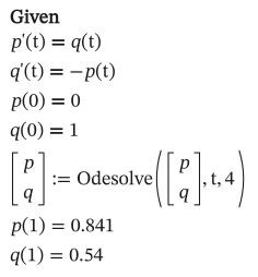
A system names its unknowns in a vector, one equation each:

As text

given
p'(t) == q(t)
q'(t) == -p(t)
p(0) == 0
q(0) == 1
[p; q] := Odesolve([p; q], t, 4)
p(1) = ?
q(1) = ?

Open this example · Download .bbm

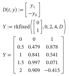
rkfixed and Rkadapt: a table of values

These take the derivatives as a function D(t, y) of a vector y, and return a matrix: the first column is t, then one column per unknown.

As text

D(t, y) := [y[1]; -y[0]]
Y := rkfixed([0; 1], 0, 2, 4, D)
Y = ?

Open this example · Download .bbm

rkfixed(y0, t1, t2, n, D) takes n equal steps (fourth-order Runge–Kutta); Rkadapt gives the same n points, with smaller steps between them where the solution needs them.

Odesolve takes starting values at one point; conditions at both ends of the range (a boundary-value problem) aren’t supported.