Plots

A plot draws one or more curves against a variable. It sees the definitions above it, like any statement there.

Insert one

Press @ on an empty spot of the page, choose Insert → X-Y plot, or click the plot button on the Insert palette. A working example appears (a sine wave), open as its settings, which are a few lines of text:

x: 0 .. 2*π
traces:
  - y: sin(x)
    label: sin(x)
axes:
  x: { grid: true }
  y: { grid: true }

Change them, then press Escape (or click elsewhere) to draw the plot. Click the plot again to change it.

A function of x

L := 6 m
q := 12 kN/m
M(x) := q*x*(L - x)/2
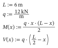
V(x) := q*(L/2 - x) — As text
L := 6 m q := 12 kN/m M(x) := q*x*(L - x)/2 V(x) := q*(L/2 - x)
Open this example · Download .bbm

title: Moment and shear
x: x = 0 m .. L
x_unit: m
traces:
  - y: M(x)
    unit: kN*m
    label: Bending moment
  - y: V(x)
    unit: kN
    label: Shear
    axis: right
    style: { line: dash, color: red }
axes:
  y: { grid: true }

x: x = 0 m .. L names the variable and its range. Without a name (x: 0 m .. L) the variable is x. The curve is sampled at 200 points by default (samples: 500 for more).
Each trace’s y is worked out at every x. unit sets the unit it is drawn in; the axis label shows it.
axis: right puts a trace on a second y axis, with its own unit.
A point that can’t be worked out (a division by zero) leaves a gap in the curve.

Data

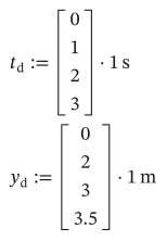
To plot measured points, give vectors of the same length for x and y:

t_d := [0; 1; 2; 3]*1 s
y_d := [0; 2; 3; 3.5]*1 m — As text
t_d := [0; 1; 2; 3]*1 s y_d := [0; 2; 3; 3.5]*1 m
Open this example · Download .bbm

x: t_d
traces:
  - y: y_d
    label: Measured
    style: { line: none, marker: circle }

A stepped range plots at exactly its values: x: x = 0, 1.5 m..L.

Axes

Under axes:, each of x, y and y2 (the right axis) can take:

Setting	Does
`min`, `max`	The ends, in the axis’s unit (otherwise they fit the data)
`step`	The distance between ticks
`log: true`	A logarithmic scale; a sampled x range is then spaced evenly in log
`grid: true`	Grid lines
`label`	The axis’s label, instead of the trace’s name and unit

title: Low-pass filter
x: f = 1 Hz .. 100 kHz
x_unit: Hz
traces:
  - y: 1/sqrt(1 + (f/(100 Hz))^2)
    label: Gain
axes:
  x: { log: true }
  y: { log: true, min: 0.001 }

Line styles

style takes line (solid, dash, dot or none), marker (none, circle or square) and color (blue, red, green, orange, purple, black, gray, or #rrggbb).

Parametric curves

A trace with an x of its own draws (x, y) as the plot’s variable runs:

title: Ellipse
x: t = 0 .. 2*π
traces:
  - x: 3 m*cos(t)
    y: 2 m*sin(t)

Size

Select a plot (drag a rectangle around it, or Ctrl+click it) and drag the handle at its bottom-right corner. Right-click a plot for Copy as image, to paste it into another program.